Intuitive intro to RL from scratch

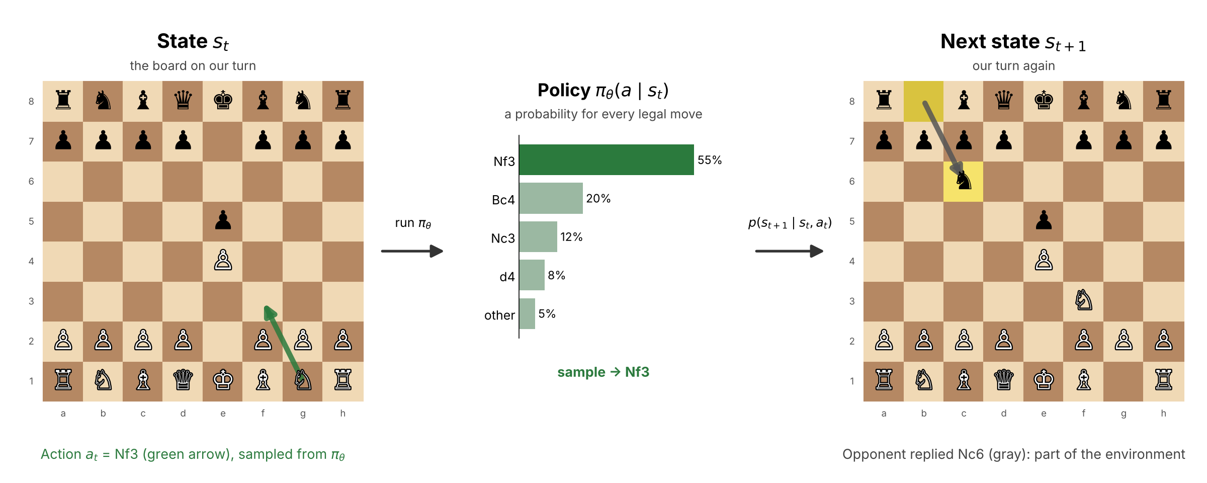
I’ll use chess as our example. We’ll play white, and treat our opponent as part of the environment.

Our strategy. In a game:

• each board position on our turn is a state $s_t$
• the move we make there is an action $a_t$

Our strategy for playing is called a policy, $π$. Given a board, it doesn’t pick one fixed move. $π(a | s)$ is a probability distribution over the legal moves. In the opening it might say “60% e4, 30% d4, 10% something else,” and we sample from that.

We can model this with a neural net: the board state goes in, it outputs a score (logit) for each move, and a softmax turns those into probabilities. We’ll call the network’s weights $\theta$ and write the policy as $\pi_\theta$ Making the policy better means changing $\theta$.

Our goal. Find the best policy: the one that wins the most games.

Rewards. To tell the policy how it’s doing, the environment hands us a number after every move, a reward $r(s_t, a_t)$. Our score for a whole game is the sum of the rewards we collected along the way.

In chess, this looks a little strange. Every move we make gets a reward of 0, except the last one: +1 if we win, -1 if we lose, 0 for a draw.

Why not reward good moves along the way, like +1 for capturing a piece? Because the policy will optimize exactly what we reward, not what we meant. Reward captures, and it’ll happily grab pieces all the way into checkmate. The only thing we actually care about is winning, so that’s the only thing we reward.

Since we sample our moves and the opponent varies, the same policy will win some games and lose others. So we can’t maximize the reward of one game. Instead we maximize the expected total reward, averaged over all the games our policy might play.

Let’s call one full game a trajectory, the sequence of boards and moves we went through:

Which game we end up playing is random. It depends on what our policy samples and how the opponent replies. Its probability is:

In words: the chance of the starting board, times the chance we picked each of our moves, times the chance the opponent replied the way they did. Only the middle term depends on our policy.

The total reward of one game is:

which in chess is just the final result, +1, −1, or 0, since every other reward is 0.

Our objective is the expected value of that over all the games our policy might play:

So finding the best policy is just finding the weights that maximize it:

Ok so what’s the most natural thing to do? We have a function we’re trying to maximize, and some current weights $\theta$. Gradient ascent says take a step in the direction of the gradient. So we need

That tells us how to move each parameter of $\theta$ to get closer to $\theta^*$.

Writing the expectation out. In chess there are finitely many possible games, so “expected reward” literally means: go through every possible game, and weigh its result by how likely our policy is to play it:

Taking the gradient. To improve the policy, we want the direction to move $\theta$ that increases $J$.

This is correct, but useless as written. We can’t sum over every possible chess game. The usual way out is to sample games and average, but that only works for an expectation. We can’t estimate this well since its literally summing over all the games. But, maybe we can try to turn this into an expectation.

This identity can help us do so. From the chain rule, $\nabla \log p = \frac{\nabla p}{p}$, so:

Substituting it in:

It’s an expectation again, so we can estimate it by playing games and averaging. But first we can simplify the thing inside the expectation. $p_\theta(\tau)$ is a product of probabilities, so $\log p_\theta(\tau)$ is a sum, and only the terms where we pick a move depend on $\theta$.

Take the log of the trajectory probability we wrote earlier:

The starting board and the opponent’s moves don’t depend on our weights, so their gradients are zero:

Plug that in, and write $R(\tau)$ as the sum of rewards:

Now we can estimate this by sampling $N$ trajectories or games from our current policy $p_\theta(\tau)$. I’ll write a superscript $(i)$ for the boards and moves from the $i$-th sample:

To compute the gradients, remember $\pi_\theta$ is some neural network we can do backpropagation on to compute the gradients. Also, $R(\tau^{(i)})$ is just $1$ if we win, $0$ if draw, and $-1$ if lose. So computing this is doable.

Then we take a gradient-ascent step, with step size $\alpha$:

That gives us our first algorithm!

REINFORCE, the vanilla policy gradient. Repeat:

1. Play $N$ games with the current policy $\pi_\theta$, recording every board $s_t^{(i)}$, move $a_t^{(i)}$, and final result $R(\tau^{(i)})$. Game $i$ lasts $T^{(i)}$ moves.

2. Compute the gradient:

3. Update the policy:

A useful way to read this gradient. It looks a lot like ordinary supervised learning, just with an extra $R(\tau^{(i)})$ multiplied in.

To see why, imagine we skip RL entirely and just try to copy an expert. We watch Magnus Carlsen play $N$ games, and $a_t^{(i)}$ are the moves he made. Training our network to imitate him is a classification problem: maximize the log-probability of each of his moves.

In other words, put more probability on whatever Magnus played. The gradient of this is:

I wrote the $\cdot\, 1$ on purpose. Compare it to our policy gradient:

They’re the same formula. The only differences: the moves come from our own games instead of Magnus’s, and each game is weighted by its result instead of by 1.

So the policy gradient is just imitation learning on our own games:

• Won ($R = +1$): imitate ourselves. Make those moves more likely.
• Lost ($R = -1$): anti-imitate. Make those moves less likely.
• Drew ($R = 0$): ignore the game.

With Magnus, every move gets weight 1 because we trust that all his moves are good. With our own games we can’t, so we let the result decide.

What’s wrong with REINFORCE? Let’s go back to playing our own games, with no expert to copy.

Look at what the gradient actually does: every move in a game gets the same weight, the final result. That’s a very blunt way to hand out credit.

Say we play a sloppy game, full of bad moves, and we’re about to get mated. Then our opponent misses a mate in one, and we win. REINFORCE gives every one of our moves +1, including all the bad ones. It works the other way too: we play a brilliant combination on move 15, blunder our queen on move 30, and lose. That brilliant move gets −1.

Over enough games this evens out. Good moves win more often than bad ones on average, so the gradient points the right way in expectation. But any single game is a very noisy signal, so we need a huge number of games before the noise averages out.

So the question for the rest of this post: instead of weighting every move by the final result, can we find a better weight for each move, one that reflects how good that move actually was?

A better weight: how much did this move help? What we really want to know about a move isn’t “did we win the game?” but “did this move make our position better or worse?”

Chess players already have a tool for this: the evaluation of a position. Is white winning, losing, or equal? Let’s make that precise.

The value of a position is the expected result of the game if we’re in state $s_t$ and keep playing with our policy from there:

It’s like an engine eval, with one difference: it measures how well our policy will do from here, not how good the position is in principle. Up a queen is +0.95 for a strong policy, but maybe only +0.3 for one that tends to blunder it back.

The Q-value is the same thing, but for a specific move: the expected result if we play move $a_t$ in position $s_t$, then keep playing with our policy:

The difference between them is the advantage:

That’s exactly the number we wanted: how much better is this move than what we’d typically play here? Positive means the move improved our chances, negative means it hurt them.

Now swap it in for the game result:

Back to our sloppy game: the bad moves now get negative weight, because each one made the position worse, even though we went on to win. The brilliant combination in the lost game gets positive weight, because it improved the position, even though we blundered later.

Of course, this assumes we know the values and Q-values, and we don’t. We’ll have to estimate them, and that comes with a tradeoff: good estimates give each move a much less noisy weight, so we need far fewer games. But if our estimates are wrong, they’ll push the policy in the wrong direction, no matter how many games we play.

Grading a move with only $V$. The advantage $A = Q - V$ needs two things we don’t know, but we can get away with just $V$.

After we play $a_t$, the opponent replies and we land in a new position $s_{t+1}$. So a natural way to grade our move is to compare how good things looked before it to how good they look after:

If the evaluation went up, the move helped. If it went down, it hurt. For the final move there’s no next position, so “after” is just the actual result: $A^{\pi}(s_T, a_T) \approx R(\tau) - V^{\pi}(s_T)$.

Why "$\approx$"? The opponent could have replied in many ways, and we’re only using the one they actually played. We don’t know how the opponent chooses their moves, and we don’t need to: their real reply is a sample from that distribution, so across many games the average takes care of itself. It’s still a sample, but a much smaller one than before. In REINFORCE, each move’s weight depended on everything that happened for the rest of the game. Now it depends on a single reply.

(In environments with rewards along the way, you’d also add the reward the move earned: $r(s_t, a_t) + V^{\pi}(s_{t+1}) - V^{\pi}(s_t)$. Chess doesn’t have any until the end.)

This is the key step. To grade every move we play, all we need is something that can evaluate a position, or have some estimator function for $V^{\pi}$

Estimating the value. So how do we get $V^{\pi}(s)$? By definition, it’s the average result when we start from position $s$ and play the rest of the game with our policy. The most direct way to estimate it is to do exactly that: put ourselves in position $s$, play the game out many times, and average the results.

This is called a Monte Carlo estimate, and it’s correct on average. With enough games it would work, but in chess “enough” is enormous. After the first few moves, almost every position we reach is one we’ll never see again, so we’d have to replay many games from every single board in every game just to grade our moves. That’s far more games than we’d ever want to play.

Instead, we can train a second neural network $\hat{V}_\phi(s)$, with its own weights $\phi$, to predict the result from the position. The training data comes free with the games we’re already playing: every position in a game gets labeled with how that game ended. We train it with a loss like squared error, which pushes its prediction toward the average result from positions like this one, exactly what $V$ is.

Each label on its own is noisy, the same problem as before: a bad position from a game we happened to win gets labeled +1. But the network sees thousands of similar positions, so it learns the average outcome from boards like this one. It has never seen this exact position, but it has seen many like it. In a sense, it’s still a Monte Carlo estimate, just averaged across similar positions instead of the same one.

We call this network the critic, because its job is to judge positions based on our current policy $\pi_\theta$. The policy network $\pi_\theta$ is the actor, because its job is to play. The actor plays games, the critic learns from how they turned out, and then the critic grades every move the actor made:

So now we have a new algorithm!

Actor-critic. Putting it all together. Start with an actor $\pi_\theta$ and a critic $\hat{V}_\phi$ (both can start random), then repeat:

1. Play $N$ games with the current actor $\pi_\theta$.

2. Grade each move with the critic, by how much it changed the evaluation. If game $i$ has $T_i$ moves:

3. Update the actor, weighting each move by its grade:

4. Update the critic on the new games. Label every position $s_t^{(i)}$ with how its game ended, $R(\tau^{(i)})$, and take a few gradient steps on the squared error between the critic’s prediction and that result:

where $\beta$ is the critic’s learning rate. Positions from games we won get pulled toward +1, from games we lost toward −1, and the critic ends up predicting the average for each kind of position. Next round, it grades moves a little more accurately.

It’s the same as REINFORCE, with one change: each move is weighted by “did it improve our position?” instead of “did we win the game?”

Ok so theres a problem with the algorithm here.

The critic is chasing a moving target. The critic is supposed to predict $V^{\pi}$, the value of a position under our current policy. But every round, step 3 changes the policy, so the thing the critic is trying to predict changes too. A position that was worth +0.2 for last round’s actor might be worth +0.4 for this round’s, because the new actor converts it better. So when the critic grades this round’s moves, it’s using estimates for a slightly older version of us.

It turns out this works anyway, as long as the actor changes slowly. With a small step size $\alpha$, the policy only shifts a little each round, so last round’s values are still close to right, and the critic, retrained every round on fresh games, keeps catching up. It’s like a coach whose read on your game is always a week behind: still useful, as long as you aren’t changing your whole style every week.

If the actor changes too much in one step, the critic’s grades go stale and the actor learns from bad advice.