This is a follow-up to my previous post, where I said I wanted to benchmark a naive Hugging Face transformers server against vLLM and understand why the performance differs.
Goal
Measure how much faster (or not) vLLM is compared to a simple baseline transformers server, and explain the gap in terms of system behavior.
Setup
- Model:
Qwen2.5-7B-Instruct - Hardware:
NVIDIA A40
Things we will measure / understand better
When I refer to request here, I’m talking about a prompt as input and the full LLM result as the output. Just like a standard request made to any LLM. Here are the charts we will measure for both naive and vLLM
- concurrency vs decode throughput (excluding the first output token per request)
- If the inference server sees 1 client, what is the total decode tokens / sec across all users (excluding each request’s first output token)
- what about 2 requests, 4 requests, 8 requests, … 128 requests.. is the work being batched well, will this work be done efficiently?
- latency vs throughput
- Use the same concurrency (number of requests) to get different points, but here we’re measuring latency (p50 and p99 time taken to finish request across all 2^n requests) vs. throughput (output tokens / sec across all requests)
- The motivation for this is to see with a fixed latency t seconds, how much throughput can we expect to get and does that change as t changes?
- concurrency vs TPOT and concurrency vs TTFT
- TTFT is time to first token
- TPOT is average time per output token excluding the first token so (latency for a request - TTFT) / (output tokens - 1)
- Use the same concurrency of varying 2^n requests..
- prompt length vs TTFT
- Does the size of the input affect the TTFT?
Okay so first let’s try to make predictions on these.. and to do this we need to look at the architecture of the LLM and do some computations.
Here are the key model values I am using (from the model config / card):
num_hidden_layers:28hidden_size(embedding size):3584num_attention_heads:28num_key_value_heads:4intermediate_size(MLP width):18944vocab_size:152064- Total parameters:
~7.6B
Qwen2.5-7B Decoder Layer Compute
Per-token flow: embedding -> 28 decoder layers -> final RMSNorm + LM head.
If the embed does not load, open it directly: Open architecture page
So before doing these computations I realized this, along with most of the modern LLM’s used something called grouped query attention (GQA). This basically saves space on the KV cache cause it forces groups of query heads to use the same k and v vectors. The way to think about it that helped me was that it’s kind of a middle ground between Multi-headed attention (MHA) where each head has its own Q K and V matrices, and Multi-Query attention (MQA) where all the Q heads share one k and v vector. MQA sacrifices on quality since these q heads are supposed to kind of understand different aspects of a sentence, but since all those q heads share the same k and v vectors per token they lose some independent perspective.. GQA is a middle ground where it turns out in MHA some groups of heads may actually need to learn the same thing, so grouping those heads together allows them to share one KV pair, so the model can use less parameters in the K and V matrices.
Computed values
1) KV bytes used on GPU to store per token
- How I compute it:
KV bytes/token = num_layers * kv_head_dim * num_kv_heads * 2 (K and V) * 2 bytes (bf16) = 28 * 128 * 4 * 2 * 2 = 57,344 bytes/token - Value:
57,344 bytes/token(~56 KB/token)
2) Weight bytes read per decode
- How I compute it: In each decode step, we read essentially all model weights for a forward pass. I ignore embedding-table bandwidth here because it is lookup-based and relatively small.
Weight bytes/decode ~= (total params - embedding params) * 2 bytes (bf16) ~= (7.6e9 - 152,064 * 3,584) * 2 ~= 1.4e10 bytes - Value:
14,000,000,000 bytes(14 GB) per decode step
3) Ridge point of A40
- How I compute it: From the NVIDIA A40 datasheet, peak dense bf16 tensor-core throughput is
149.7 TFLOP/sand memory bandwidth is696 GB/s.
If operational intensity is above this, decode is compute-bound; otherwise it is memory-bound.Ridge point = peak FLOP/s / memory bandwidth (bytes/s) = (149.7e12) / (696e9) ~= 215 FLOP/byte - Value:
~215 FLOP/byte
Notation used below:
B: batch size (number of sequences decoded in parallel)T: number of tokens already in the context per sequence (at this decode step)
4) Bytes moved per decode step
- How I compute it: In one decode step, we move weight bytes (from #2) plus KV-cache bytes for all prior tokens across the batch.
Bytes/decode = weight_bytes + B * T * kv_bytes_per_token = 14,000,000,000 + B * T * 57,344 - Value:
14,000,000,000 + 57,344 * B * T bytes
5) FLOPs per decode step
- How I compute it: I use
2*m*nFLOPs for each matrix-vector multiply and sum attention + MLP + LM-head terms.FLOPs/decode = attention FLOPs + MLP FLOPs + LM-head FLOPs = (num_layers) * B * (Q_proj_flops + K_proj_flops + V_proj_flops + O_proj_flops + attention q dot k + attention weighted sum of v) + (num_layers) * B * (gate_flops + up_flops + down_flops) + LM_head_flops = 28*B*((2*3584^2 + 2*3584*512 + 2*3584*512 + 2*3584^2) + 28*T*(128 + 128) + 28*T*(128 + 128)) + 28*B*(2*3584*18944 + 2*3584*18944 + 2*3584*18944) + B*2*3584*152064 ~= B * (1.4e10 + 4.0e5 * T) - Value:
B * (1.4e10 + 4.0e5 * T) FLOPs
6) Max concurrent sequences that fit in memory
-
Define variable:
S: tokens reserved per sequence in KV cache (prompt tokens + generated tokens budget)
-
How I compute it: Max concurrent sequences is available KV memory divided by KV bytes required per sequence.
max_concurrent_sequences
= free_kv_memory_bytes / (S * kv_bytes_per_token)

free_kv_memory_bytes
~= 48 GB * 0.9 - weight_memory
~= 28 GB

max_concurrent_sequences
~= 28,000,000,000 / (S * 57,344)
~= 488,281 / S
This approximation assumes
28 GBis already net KV-cache budget (after weights and runtime overhead), with no fragmentation penalty. -
Value:
~488,281 / Ssequences
Ok so now since we’re actually comparing vLLM vs HF baseline and making predictions on how much faster one will be than the other, we first need to understand how these inference servers work
Main differences
| Aspect | HF baseline | vLLM |
|---|---|---|
| Scheduling | One request at a time, under a lock. Others wait. | Continuous batching: many requests share each step, and the batch changes every step. |
Batch size B | Always 1 | Up to min(C, capacity, max-num-seqs) |
| KV cache memory | One cache per request, grown as tokens are added, thrown away when the request ends | One big pool of fixed-size blocks, allocated at startup and handed out to requests as needed (PagedAttention) |
| Sharing KV | None | Prefix caching: requests with the same prefix share blocks and skip that prefill |
| Long prompts | Prefilled in one go | Chunked prefill: split across steps, mixed with other requests’ decode |
| Per-step overhead | A Python loop in generate(), launching every kernel individually | CUDA graphs replay the step with one launch; scheduling runs apart from the GPU loop |
| Kernels | PyTorch SDPA (which can use FlashAttention internally) | Optimized attention backends, fused ops |
Explaining each difference
1) Scheduling
https://www.usenix.org/conference/osdi22/presentation/yu This is a famous relevant paper that explains this idea. There are two ideas here implemented in vLLM : iteration-level scheduling and selective batching. I found the video pretty well-explained.
With iteration-level scheduling, the scheduler can rebuild the batch at every decode step: if capacity opens up, a waiting request can join immediately in the next iteration.
There’s one problem with this, in that when we’re computing the attention layer we cant do all of these together in one batch since the kv cache is different for requests in different sequences. Each sequence attends to its own kv cache. Batching can happen safely in every other part of the model. So the case of attention we split the tensors up, compute attention for each, and merge the outputs together. This is known as selective batching.
So back to our experiment: to better mimic real inference servers, I’ll add a small jitter so requests arrive at slightly different times instead of all at once. I originally thought iteration-level scheduling might not matter here because we fix output tokens in every test, which can make many requests start in the same batch and finish around the same time. The jitter also helps us verify whether iteration-level scheduling still provides gains in this more controlled setup.
2) Batch size B
HF uses B = 1, so combined with the fact that it uses request-level schedling not iteration-level we can only do one request at a time. However vLLM can use B up to min(C, capacity based on memory, max-num-seqs). Note the capacity based on memory changes, but we’ll get into that in KV cache memory.
3) KV cache memory
Here, vLLM uses the concept of pagedAttention. Here is a good video on it https://www.youtube.com/watch?v=UdNocRPQS3Y . Essentially kv cache space is split into small fixed-size blocks which are each meant to store the k and v vectors for a few tokens. Each sequence still sees a logically contiguous KV cache, but physically it is backed by non-contiguous blocks, and a block table mapping tracks the order. Once one block is filled up, vLLM allocates a new one and appends it through that mapping. This helps reduce fragmentation and wasted memory, makes KV growth easier as sequences extend, and also enables better sharing/reuse such as prefix caching.
In the naive decode implementation we’re using, KV growth can require re-allocating a larger KV buffer for a sequence and copying the old cache into it, instead of only appending into pre-allocated blocks. That extra copy sounds expensive, but decode already streams about ~14 GB of weights per step, so KV-copy traffic is usually much smaller in comparison (and GQA further reduces KV size).
For example, using our 57,344 bytes/token estimate and T = 512 tokens:f
KV copy bytes per step ~= 57,344 * 512 * 2 = 58,720,256 bytes (~56 MB), which is << 14 GB
4) Sharing KV
Ok so usually in pagedAttention, the KV cache blocks will be shared if the prefix is shared since that means the k and v vectors are the same up until the token. However we’re using random prompts so this probably will barely matter for us.
5) Long prompts
Here is the original paper on chunked prefill: https://arxiv.org/pdf/2403.02310
With long prompts, prefill is compute-heavy and can dominate a batch, which increases latency for ongoing decode requests. Chunked prefill avoids that by splitting prefill into smaller chunks and scheduling those chunks across iterations, interleaved with decode work from other requests. This keeps decode latency more stable while still making progress on long-prefill requests.
In each scheduling step, decode tokens are prioritized first, and any remaining token budget is used for chunked prefill. When max_num_batched_tokens is set well above max_num_seqs, prefill usually still gets budget each step, so starvation is less likely (though still possible under sustained decode-heavy load).
As for the token budget default we’re using for vLLM it depends on the version. Let’s use v0.30.0, the most recent one. Since we’re using the A40, the default max_num_batched_tokens is 2048 and the max_num_seqs is 256.
6) Per-step overhead
This part refers to host-side overhead (Python scheduling, kernel launches, and synchronization) that can leave gaps where the GPU is not fully utilized. A useful approximation is:
step time ~= GPU compute time + launch/scheduling overhead
Some overlap can happen, so this is not exact, but it is a good mental model.
In the naive path, this overhead is paid very frequently and is not spread out because each step does relatively little batched work. In vLLM, CUDA graph replay plus more optimized/fused execution reduces launch overhead and idle gaps, so per-step overhead is usually lower. At concurrency 1, the overhead gap is often smaller than at high concurrency, but not necessarily zero.
Predictions
Now that we have a sense of the main differences between our inference engines, let’s make predictions for the graphs.
1a) Concurrency vs decode throughput (512 input tokens, 128 output tokens)
For chart 1, throughput means decode throughput only: total generated tokens/sec excluding the first output token of each request.
At C = 1, scheduling and batching should not make much difference between the naive approach and vLLM, since there is only one sequence. For KV-cache traffic, B is small enough that in 14,000,000,000 + 57,344 * B * T bytes per decode step, the 14 GB weight term still dominates, so we should not expect a large gap from KV movement alone. Since this chart excludes the first output token, prefill effects are mostly excluded from this metric as well. The main difference at C = 1 should come from per-step overhead (where vLLM benefits from CUDA graph replay after warmup). Let the decode-throughput ratio at C = 1 be r.
At C = 2, the same logic still applies, but now B = 1 in the naive setup matters because it cannot batch requests. So the expected decode-throughput ratio becomes approximately 2 * r.
This trend should continue as C increases, until KV-cache movement becomes large enough to impact latency. Using T = 512 as an approximation (actual decode steps are between 512 and 512 + 128), KV-cache bytes per step are:
57,344 * 512 * B
So:
C = B = 32->0.93 GBC = B = 64->1.88 GBC = B = 128->3.76 GB
At that point, KV movement is no longer negligible, which matters because we are still memory-bound. So I expect vLLM decode throughput to scale roughly like r * C at first (on a log-scale concurrency axis, this appears close to exponential), then flatten somewhat at higher C as KV-memory movement starts to take a real toll in the naive approach.
1b) Concurrency vs decode throughput (8192 input tokens, 128 output tokens)
Okay as im working the math out and writing this out, I’m spending too much time on these predictions I thought it would be easier but there are so many more factors than I thought.. Also it could totally be that I’m very off on this. I’m going to time box this and just generate the first graph and see if it matches my prediction… May continue the other ones in a separate blogpost
Here’s a repo I created with Claude to run on the A40 server:
Warmup and runtime notes (vLLM)
GPU and model memory
- vLLM reported
44.42 GiBtotal and44.16 GiBfree device memory at startup. - The A40 is sold as
48 GB; this is the usable amount after driver/runtime reserve. - Later memory breakdown:
- weights + non-torch memory:
15.55 GiB - peak activation memory:
1.44 GiB - CUDA graph memory:
0.24 GiB
- weights + non-torch memory:
Scheduler/runtime settings used for the sweep
- Prefix caching:
on - Chunked prefill:
on - Max batched tokens:
2048 - Attention backend:
FlashAttention 2 - KV cache:
22.99 GiB(430,528tokens)
I guess I was wrong about the KV cache, there’s less memory availabel than I thought.
First measured result: chart 1a
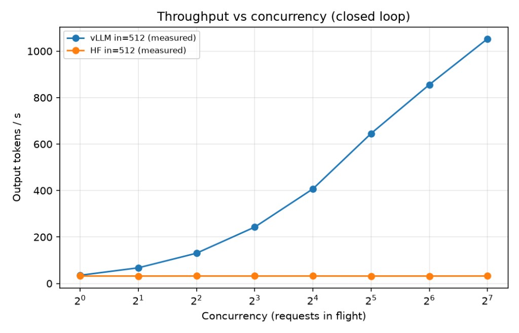
At 2^0 concurrency (C = 1), overhead differences look minimal in this run, so vLLM and the HF baseline are very close at that first point. So theres probably not much overhead
You can see the full raw result values in the results folder.
This only cost $1.12 to run all of it.
References
- vLLM Documentation
- Hugging Face Transformers
- vLLM OSDI’22 Paper/Presentation (USENIX)
- PagedAttention explainer video
- Chunked Prefill paper